Project Report

BillionaireOmics: Decoding the World’s Richest

Pei Tian, Mengxiao Luan, Sitian Zhou, Yuzhe Hu, Shuchen Dong

knitr::opts_chunk$set(message = F, warning = F)

# Library Import Here!!!!!
library(tidyverse)
library(leaflet)
library(sf)
library(rnaturalearth)
library(plotly)
library(readxl)
library(janitor)
library(forcats)
library(ggpubr)
library(dplyr)
library(ggplot2)
library(multcompView)
library(rvest)
library(httr)
library(fuzzyjoin)
library(readr)
#library(car)
#library(carData)
#library(MASS)
library(qqplotr)

theme_set(
  theme_minimal() +
  theme(plot.title = element_text(hjust = 0.5),
        text = element_text(family = "Helvetica")
  )
)

Introduction

Motivation

In this project, our goal is to gain a comprehensive view of billionaire wealth dynamics. We are interested in the geographic distribution of billionaires worldwide and how their net worth changes over time and among diverse demographic groups. Furthermore, we want to explore implications for wealth distribution and economic conditions. Finally, we plan to conduct some statistical tests and linear regression to identify potential factors contributing to the success and accumulation of wealth among billionaires.

Related work

The Forbes updates the World’s Billionaire List annually, which inspired us to pool together the data from the past decade and explore if there are any trends in their wealth across years or among diverse demographic groups. Moreover, understanding the wealth distribution of the richest also helps gain a picture of the global economy. There has always been discussions about whether or not billionaires have positive effects on the economy (J. Svejnar, 2015; J. Flanigan& C. Freiman, 2022). This further makes us curious about what makes them billionaires and what factors contribute to their accumulation of assets.

Initial questions

• How has billionaires’ wealth changed in the past decade?
• What are the geographical distribution as well as the demographic characteristics of billionaires of billionaires?
• What are some potential factors that contribute to billionaires’ success?

Data cleaning

Country code

The country code dataset contains country names along with their corresponding standard two-letter, three-letter, and numeric codes. The dataset can be accessed here.

In cleaning this dataset, we renamed some countries to make them consistent with the naming in other datasets. We then selected variables that are useful for downstream analysis.

country_code <-
  read_csv("../data/raw/country_code.csv") |> 
  clean_names() |> 
  rename(
    "country_name" = "english_short_name_lower_case"
  ) |> 
  mutate(
    country_name = recode(country_name, 
                          "United States Of America" = "United States",
                          "Virgin Islands, British" = "British Virgin Islands",
                          "Korea, Republic of (South Korea)" = "South Korea",
                          "Virgin Islands, U.S." = "U.S. Virgin Islands",
                          "Tanzania, United Republic of" = "Tanzania",
                          "Turks and Caicos" = "Turks and Caicos Islands",
                          "Macao" = "Macau")) |> 
  select(country_name, alpha_3_code)

Billionaires 2010-2023

The raw dataset contains information on global billionaires from 1997 to 2023. It offers a glimpse into the distribution of wealth, industries of operation, and demographic profiles of billionaires on a global scale. The dataset is available here.

The data prior to 2010 contains too many missing values, so we decided to filter for the data after 2010. We then removed any special characters or letters in net_worth and industries variables and converted the net_worth variable to numeric. Additionally, we identified discrepancies in data entry where values were incorrectly or inconsistently recorded; we recoded those values for consistency. Finally, we removed unused variables and merged the dataset with the country_code dataset for further analysis.

bil_2010_2023 <-
  read_csv("../data/raw/billionaires_1997_2023.csv") |> 
  filter(year >= 2010)

bil_2010_2023_clean <-
  bil_2010_2023 |> 
  mutate(
    net_worth = str_replace_all(net_worth, " B", ""),
    net_worth = as.numeric(net_worth), 
    industries = str_replace_all(business_industries, "[\\['\\]]", ""),
    country_of_residence = 
      recode(country_of_residence, 
             "Eswatini (Swaziland)" = "Swaziland",
             "Scotland" = "United Kingdom",
             "Czechia" = "Czech Republic",
             "Hong Kong SAR" = "Hong Kong"),
    industries = 
      recode(industries,
             "Fashion and Retail" = "Fashion & Retail",
             "Finance and Investments" = "Finance & Investments",
             "Food and Beverage" = "Food & Beverage",
             "Healthcare" = "Health care",
             "Media" = "Media & Entertainment")) |> 
  left_join(country_code, c("country_of_residence" = "country_name")) |> 
  select(-c(month, rank, last_name, first_name, birth_date, business_category,
            business_industries, organization_name, position_in_organization))

Billionaires 2023 with GDP data

The billionaires 2023 dataset includes statistics on global billionaires, such as information about their wealth, industries, and personal details. This dataset also contains more detailed country information of which each billionaire resides, which is useful for the following analysis. The dataset is available here.

Similar as the cleaning steps for the previous dataset, we removed the special character, $, in the gdp_country column and converted it to numeric. We then converted the unit of net_worthand gdp_country to billions and trillions, respectively. Furthermore, we modified gender variable, changing letters “M” and “F” to words “Male” and “Female”. Last, we renamed and selected useful variables.

bil_gdp_2023 <-
  read_csv("../data/raw/billionaires_2023.csv")

bil_gdp_2023_clean <-
  bil_gdp_2023 |> 
  clean_names() |> 
  mutate(
    net_worth = final_worth / 1000,
    gdp_country = str_replace_all(gdp_country, "[$,]", ""),
    gdp_country = as.numeric(gdp_country) / 1e12,
    gender = 
      case_match(
        gender,
        "F" ~ "Female",
        "M" ~ "Male")) |>
  select(net_worth, full_name = person_name, age, gender, 
         country_of_citizenship, country_of_residence = country, 
         city_of_residence = city, industries, self_made, cpi_country, 
         cpi_change_country, gdp_country, life_expectancy_country)

Region-level GDP

The GDP dataset encompasses GDP information spanning 262 distinct countries or regions from 1960 to 2022. The dataset can be downloaded here.

For this dataset, we filtered the data starting from 2010 and converted the unit of GDP to trillions. We then selected and renamed some variables.

country_gdp <-
  read_csv("../data/raw/country_gdp.csv")

country_gdp_clean <-
  country_gdp |> 
  filter(year >= 2010) |> 
  mutate(gdp = value / 1e12,
         name = country_name, 
         code = country_code) |> 
  select(name, code, year, gdp)

Supplementary dataset

Given the issue that the region Taiwan is missing GDP data in raw dataset, we used a supplementary dataset to remedy it.

The Taiwan GDP data can be accessed here. This table contains Taiwan GDP data from 1960 to 2022.

Since the data is solely accessible through the website, we wrote a function to extract the data. We then cleaned up the gdp variable, extracted data starting from 2010, and removed unused variables. Finally, we combined Taiwan GDP data with the main GDP dataset.

fetch_tw_gdp = function(){
  url = "https://countryeconomy.com/gdp/taiwan"
  tw_gdp_html = read_html(url)
  mydata <- tw_gdp_html|> html_table()
  return(mydata[[1]])
}

extract_gdp = function(string){
  str_vec = str_extract(string, "\\d*,\\d*") |> 
    str_split(",") |> 
    nth(1)
  s = ""
  for(e in str_vec){
    s = str_c(s, e)
  }
  return(s)
}

tw_gdp = fetch_tw_gdp() |>
  janitor::clean_names() |>
  mutate(gdp = map(annual_gdp_2, extract_gdp) |> as.numeric(),
         year = date |> as.numeric(), 
         name = "Taiwan, China",
         code = "TWN",
         gdp = gdp/1e6) |>
  filter(year >= 2010) |>
  select(name, code, year, gdp)
  
  country_gdp_clean = bind_rows(country_gdp_clean, tw_gdp)

Industry-level GDP for US

This dataset contains GDP data for each industry in the US from 2017 to 2022. The dataset can be downloaded here.

After importing the data, we removed rows containing the title, headers, and unrelated information. We then renamed columns and tidied the dataset.

indus_gdp <-
  read_excel("../data/raw/usa_industry_gdp.xlsx", sheet = 18, skip = 4)

indus_gdp_clean <-
  indus_gdp |> 
  slice(3:30) |> 
  rename(
    "industries" = "...2",
    "2017" = "...3",
    "2018" = "...4",
    "2019" = "...5",
    "2020" = "...6",
    "2021" = "...7",
    "2022" = "2020...8") |>
  filter(!(industries %in% c("Finance, insurance, real estate, rental, and leasing",
                            "Educational services, health care, and social assistance",
                      "Arts, entertainment, recreation, accommodation, and food services"))) |> 
  select(industries, `2017`:`2022`) |> 
  pivot_longer(`2017`:`2022`, names_to = "year", values_to = "industry_gdp") |> 
  mutate(year = as.numeric(year),
         industry_gdp = industry_gdp / 1000)

After obtaining the tidied dataset, we wanted to merge the industry-level GDP dataset with the Billionaire 2010-2023 dataset which contains information about the business category for each billionaire. The main challenge here is that the two datasets are inconsistent in the industry naming conventions. To merge the two datasets, we first extracted industry names from the two datasets and split the industry names into keywords. We then use the function regex_inner_join(), which uses regex to match each keyword, to perform inexact matches between the datasets.

# industry names from industry_gdp_clean
df1 <- indus_gdp_clean |> select(industries) |> unique()
# industry names from bil_2013_2023_clean (only for USA from 2017 to 2022!)
df2 <- 
  bil_2010_2023_clean |> 
  filter(country_of_residence == "United States" & year >= 2017 & year <= 2022) |> 
  select(industries) |> 
  drop_na() |> 
  unique() |> 
  mutate(
    categories = industries,
    # rename some industries for better match results
    categories = recode(categories, 
                        "Technology" = "Information",
                        "Logistics" = "Transportation and warehousing")) |> 
  # extract keywords for each industry
  separate(categories, into = c("word1", "word2"), sep = " & ") |> 
  pivot_longer(
    word1:word2,
    names_to = "order",
    values_to = "keywords"
  ) |> 
  drop_na(keywords)

# use regex to perform inexact matching
reg_match <-
  regex_inner_join(df1, df2, by=c("industries" = "keywords"), ignore_case = TRUE) |> 
  distinct(industries.y, .keep_all = TRUE) |>
  # removed service industry bc it's too general
  filter(industries.y != "Service") |> 
  select(industries.x, industries.y)

Merge and output cleaned datasets

After cleaning all the datasets, we merged them into main datasets and removed redundant variables. Finally, we output the datasets for downstream analyses.

bil_gdp_2010_2023 <-
  left_join(bil_2010_2023_clean, country_gdp_clean, 
            by = join_by(alpha_3_code == code, year == year), multiple = "all") |>
  mutate(region_gdp = gdp, region_code = alpha_3_code) |>
  select(-c(gdp, alpha_3_code, name))
  
 bil_gdp_indus_usa <-
  bil_gdp_2010_2023 |> 
  filter(country_of_residence == "United States" & year >= 2017 & year <= 2022) |> 
  left_join(reg_match, c("industries" = "industries.y")) |> 
  left_join(indus_gdp_clean, c("industries.x" = "industries", "year" = "year")) |> 
  select(-industries.x, -region_code)
# save datasets
write_csv(bil_gdp_2010_2023, "../data/tidy/billionaire_gdp.csv")
write_csv(bil_gdp_indus_usa, "../data/tidy/billionaire_gdp_indus_usa.csv")
write_csv(country_gdp_clean, "../data/tidy/gdp.csv")
write_csv(bil_gdp_2023_clean, "../data/tidy/billionaire_2023.csv")

Exploratory analysis

Categorical EDA

Some exploratory data analysis can be carried out using the cleaned data, which gives us a fundamental comprehension of the data before doing statistical works like hypothesis tests and regression.

knitr::opts_chunk$set(
        echo = TRUE,
        warning = FALSE,
        message = FALSE,
        fig.width = 8, 
  fig.height = 6,
  out.width = "90%"
)

options(
  ggplot2.continuous.colour = "viridis",
  ggplot2.continuous.fill = "viridis"
)

scale_colour_discrete = scale_colour_viridis_d
scale_fill_discrete = scale_fill_viridis_d

theme_set(
  theme_minimal() +
  theme(plot.title = element_text(hjust = 0.5),
        text = element_text(family = "Helvetica")) + 
  theme(legend.position = "right"))

General wealth distribution

Focusing on the data collected in 2023, we can depict the distributions of billionaires in several categories as well as their wealth pattern.

# import data
bil_2010_2023 =
  read_csv("../data/tidy/billionaire_gdp.csv") |>
  select(-starts_with("region")) |>
  drop_na()

bil_gdp = read_csv("../data/tidy/billionaire_gdp_indus_usa.csv") |>
  select(-(age:wealth_status)) |>
  drop_na()

# filter data
bil_2023 = 
  bil_2010_2023 |>
  filter(year == 2023)

Overall wealth distribution

The overall distribution of wealth of the billionaires is right-skewed, with a few people possessing a net wealth over 100 billion dollars, which requires some transformations before further tests and analysis.

# overall distribution
wealth_distribution_1 =
  bil_2023 |>
  ggplot(aes(x = net_worth)) +
  geom_histogram() +
  labs(x = "Net wealth(billion dollars)",
       y = "Count")

wealth_distribution_2 =
  bil_2023 |>
  ggplot(aes(x = net_worth)) +
  geom_density() +
  labs(x = "Net wealth(billion dollars)",
       y = "Density")

ggarrange(wealth_distribution_1, wealth_distribution_2,
          labels = c("A", "B"), ncol = 1, nrow = 2) |>
  annotate_figure(
    top = text_grob("Overall wealth distribution of billionaires in 2023"))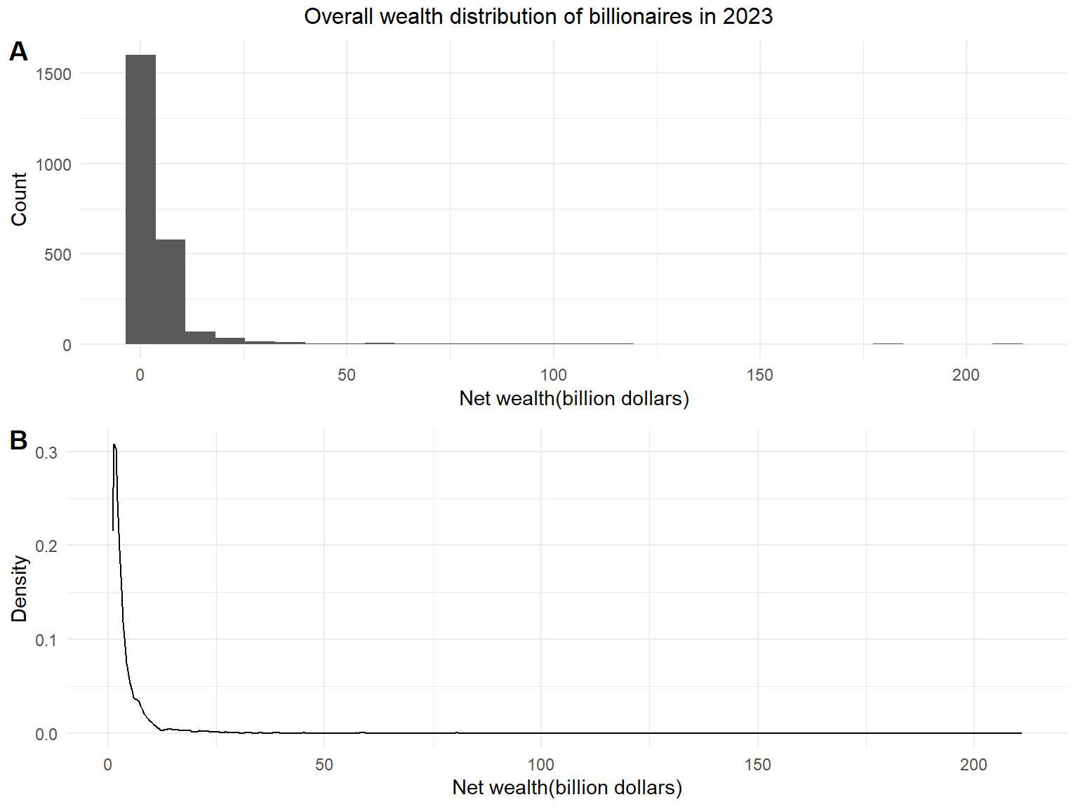

Wealth distribution in wealth groups

The skewness can be seen more clearly if we divide the billionaires into four different groups according to their net worth, where we can find a few people in the last group in possession of more than 100 billion wealth.

Wealth distribution in categorical groups

The data can be separated using categorical factors related to net worth of wealth, including approach and wealth status, which indicate whether the billionaire is self-made or not and the trend of the billionaires’ wealth amount, respectively. There are more self-made billionaires than inherited in 2023, and the majority of the population possess a decreased wealth amount. The difference in the wealth amount of different groups does not seem significant.

Demographic distribution

Divide the population into four groups based on their age, the number and wealth distribution of billionaires in each group can be delineated. The average wealth tends to increase as the group age grows, which can be tested later.

Divided by age

The age distribution is relatively symmetric and the size of the four age groups are quite close to each other. The average net wealth amount seems to be larger in groups with higher age.

# age division
billionairs_age = 
  bil_2023 |>
  mutate(
    age = 
      case_when(
        age <= 55 ~ "<=55",
        age > 55 & age <= 65 ~ "55~65",
        age > 65 & age <= 75 ~ "65~75",
        age > 75 ~ ">75")) |>
  mutate(
    age = 
      forcats::fct_relevel(
        age, c("<=55", "55~65", "65~75", ">75")))

# age visualization
age_distribution_3 =  
  billionairs_age |>
  ggplot(aes(x = age, y = net_worth)) + 
  geom_violin(aes(fill = age), alpha = 0.5) +
  labs(title = "Net wealth of different age groups",
       x = "Age of billionaires",
       y = "Net wealth(billion dollars)")

ggplotly(age_distribution_3)

Divided by gender

There are much more male billionaires than female in the year of 2023, yet the net worth in the two gender groups do not look much different.

# gender visualization
## number of people
bil_2023 |>
  count(gender) |>
  plot_ly(x = ~gender, y = ~n, color = ~gender,
          type = "bar", colors = "viridis") |>
  layout(title = "Number of billionaires of different genders",
         xaxis = list(title = "Gender"),
         yaxis = list(title = "Number of billionaires"),
         font = list(family = "Helvetica"))

Divided by country

Among all the countries listed, United States has the largest number of billionaires in both citizenship and residence.

# citizenship description
bil_2023 |>
  group_by(country_of_citizenship) |>
  summarize(mean_wealth = mean(net_worth),
            N = n()) |>
  arrange(desc(N)) |>
  slice(1:3) |>
  knitr::kable() |>
  kableExtra::kable_styling(bootstrap_options = c("striped", "hover"))

country_of_citizenship	mean_wealth	N
United States	6.465620	669
China	3.488403	457
India	4.311348	141

# residence description
bil_2023 |>
  group_by(country_of_residence) |>
  summarize(mean_wealth = mean(net_worth),
            N = n()) |>
  arrange(desc(N)) |>
  slice(1:3) |>
  knitr::kable() |>
  kableExtra::kable_styling(bootstrap_options = c("striped", "hover"))

country_of_residence	mean_wealth	N
United States	6.417758	687
China	3.567769	484
India	4.299237	131

Industry distribution

The number of billionaires from different industries also differ, with a largest proportion in the field of finance and investments. The correlation between industry and the arise of billionaires may lie in the economic development and GDP distribution of different industries, which requires further investment in longitudinal data.

# industry visualization
## number of people
bil_2023 |>
  count(industries) |>
  mutate(industries = fct_reorder(industries, n)) |>
  plot_ly(x = ~industries, y = ~n, color = ~industries,
          type = "bar", colors = "viridis") |>
  layout(title = "Number of billionaires in different industries",
         xaxis = list(title = "Industry field"),
         yaxis = list(title = "Number of billionaires"),
         font = list(family = "Helvetica"))

Comparison between years

We can compare the data across different years as well. The plot suggests a slight difference between the average wealth of all the billionaires in 2013 and 2023. Besides wealth pattern, the distribution of gender may also change over time, with an increased number of individuals in both male and female groups.

# filter data
bil_2013_2023 =
  bil_2010_2023 |>
  filter(year == 2013 | year == 2023) |>
  mutate(year = as.factor(year))

# year visualization
year_gender_distribution_2 =
  bil_2013_2023 |>
  ggplot(aes(y = net_worth, x = gender, fill = gender)) +
  geom_violin() +
  facet_grid(.~year) +
  labs(title = "Wealth distribution over gender and year",
       x = "Gender of billionaires",
       y = "Net wealth(billion dollars)")

ggplotly(year_gender_distribution_2)

Conclusion

In summary, the categorical exploratory analysis centers on data collected in 2023 and investigates the distribution of billionaires as well as their net wealth, which can be divided into three main fields: general wealth distribution, demographic distribution and industry distribution. We also compare the data in 2013 and 2023 for some difference across time.

It can be seen in the plots that the distribution of billionaires and their wealth pattern differ in some potential correlated factors such as age, gender, industry and time. Further visualizations and statistical analysis are needed to explore in depth the relationships between these variables, and a regression model may be constructed based on the results to predict the future wealth of billionaires given necessary information.

Some accessorial attempts in this process are posted on the categorical EDA page of the project, which will not be repeated here.

Longitudinal EDA

In this analysis, in two main aspects, through a series of Longitudinal visualizations, we explore the changes in national GDPs, the evolution of industry wealth, the trends in city net worth, and the distribution of billionaire wealth across different sectors, countries, regions and genders. Our insights uncover pronounced variations in economic growth, industry supremacy, urban wealth clusters, and persistent wealth accumulation disparities.

Billionaire Economic trends

GDP Trends:

Our longitudinal study spotlights the fluctuations in GDP, capturing China’s meteoric rise, the USA’s steady climb, and Japan’s stasis.

Sectoral Wealth Growth:

billionaire_gdp_indus_usa <- read.csv("../data/billionaire_gdp_indus_usa.csv")
billionaire_gdp <- read.csv("../data/billionaire_gdp.csv")
gdp <- read.csv("../data/gdp.csv")

# barplot-all industries overtime
bil_industry = 
  billionaire_gdp |> 
  mutate(industries = replace(industries, industries == "Billionaire", NA))|>
  drop_na(industries) |> 
  group_by(year, industries) |> 
  summarize(n = n()) |> 
  ggplot(aes(x = year, y = n, fill = industries))+
  theme_minimal()+
  geom_bar(position="stack", stat="identity")+
  labs(title = "Number of billionaires in different industries from 2010 to 2023", 
       x = "Year", y = "Number of billionaires", fill = "Industries")+
  scale_x_continuous(breaks = 2010:2023)+
  theme(plot.title = element_text(hjust = 0.6),
        text = element_text(family = "Helvetica")) 

ggplotly(bil_industry)

The global chart shows a clear upward trend in the number of billionaires across various industries, with significant growth in sectors such as Technology and Finance & Investments.

# barplot-US industries overtime
indus_gdp = 
  billionaire_gdp_indus_usa |> 
  drop_na(industry_gdp) |> 
  group_by(year, industries) |> 
  summarize(n = n()) |> 
  ggplot(aes(x = year, y = n, fill = industries)) +
  theme_minimal() +
  geom_bar(position="stack", stat="identity") +
  labs(title = "Number of billionaires in different industries in the USA from 2017 to 2022", 
       x = "Year", y = "Number of billionaires", fill = "Industries") +
  scale_x_continuous(breaks = 2017:2022)+
  theme(plot.title = element_text(hjust = 0.6),
        text = element_text(family = "Helvetica")) 

ggplotly(indus_gdp)

The USA-specific chart also displays an increase in the number of billionaires, particularly in Technology and Finance & Investments, while those engaged in health care increased significantly after 2020 due to the global epidemic.

# barplot-US industries overtime
data_filtered <- billionaire_gdp_indus_usa %>%
  filter(year >= 2017 & year <= 2022) %>% 
  na.omit()

gdp_industry_usa <- data_filtered |> 
  select(year, industries, industry_gdp) |> 
  unique() |> 
  ggplot(aes(x = year, y = industry_gdp, color = industries)) +
  geom_line(size = 1.2) +
  theme_minimal() +
  labs(title = "Industry GDP by year from 2017 to 2022 in the USA", 
         x = "Year", y = "Industry GDP(trillions)", color = "Industries")+
  theme(plot.title = element_text(hjust = 0.5),
        text = element_text(family = "Helvetica"))

ggplotly(gdp_industry_usa)

The chart illustrates the GDP changes of various industries in the USA from 2017 to 2022. It highlights that the Real Estate sector experienced the most significant growth, while the Media and Entertainment industry saw the least. There was a noticeable downturn in 2020 attributed to the COVID-19 pandemic, affecting billionaires across all sectors.

In a word, the Technology and Finance & Investments industries exhibit notable upward trajectories. The United States, in particular, has witnessed a surge in billionaire numbers in these sectors, with Technology and Healthcare experiencing pronounced growth, the latter propelled by the global pandemic. Real Estate, despite a universal setback in 2020 due to COVID-19, bounced back robustly, especially in the US, indicating the sector’s resilience and potential for wealth generation.

Billionaire Residency Wealth Analysis:

Additionally, we note stable rankings for cities like Medina and Omaha, while recognizing the burgeoning wealth in locales such as Austin and Seattle, which signifies a shift in the geographic distribution of affluence.

Billionaire Wealth Distribution

Global Net Worth Trends:

Global net worth rebounds from 2016 and 2020 declines, peaking in 2021, as billionaires and emerging markets thrive.

Region Wealth Comparison:

On a regional scale, the US leads in billionaire net worth, with China following but displaying fluctuations indicative of economic volatility. The consistency in Germany and the rise in India align with their respective economic narratives, while Hong Kong’s decline post-2019 suggests geopolitical and economic shifts.

Gender Wealth Gap:

The charts show a persistent gender gap in billionaire wealth, suggesting systemic barriers to entry and growth for women in the highest echelons of wealth. The trends could also reflect broader societal and economic structures that historically favor male dominance in business and wealth creation.

Self-Made Billionaires:

The examination of self-made billionaires reveals a robust majority, underscoring a trend towards wealth creation through entrepreneurship and innovation rather than inheritance.

Conclusion

To sum up, the analysis of billionaire economic trends reveals robust sectoral growth, a concerning gender wealth gap, and a resilient global wealth accumulation with regional nuances. The data points towards the necessity for inclusive policies and the potential of emerging markets, while also highlighting the transformative impact of self-made entrepreneurship on the global wealth canvas.

Geographical EDA

bil_gdp = read_csv("../data/tidy/billionaire_gdp.csv") 
bil_gdp = bil_gdp |>
  select(-wealth_status) |>
  mutate(gender = factor(ifelse(is.na(gender), "Unknown", gender)),
         year = as.integer(year),
         age = as.integer(age),
         country_of_residence = factor(country_of_residence),
         country_of_citizenship = factor(country_of_citizenship),
         region_code = factor(region_code),
         industries = factor(ifelse(is.na(industries), "Unknown", industries)),
         self_made = factor(ifelse(is.na(self_made), "Unknown", self_made))
         )

gdp_data = read_csv("../data/raw/gdp_worldbank.csv", skip = 4) |>
  janitor::clean_names() |>
  select(country_name, country_code, starts_with("x")) |>
  pivot_longer(cols = starts_with("x"), names_to = "year", names_prefix = "x", values_to = "value") |>
  mutate(gdp = value/1e12, 
         year = as.integer(year),
         name = country_name, 
         code = country_code) |>
  filter(year >= 2010) |>
  select(name, code, year, gdp)

world_polygon = ne_countries(scale = "medium", returnclass = "sf")
world_point = st_point_on_surface(world_polygon)

target_year = 2022
gdp_viz = gdp_data |>
  filter(year == target_year) |>
  left_join(world_polygon, by = join_by(code == adm0_a3)) |>
  st_as_sf()

bil_viz = bil_gdp |>
  filter(year == target_year) |>
  group_by(region_code, year) |>
  arrange(desc(net_worth)) |>  # Arrange in descending order based on 'value'
  mutate(rnk = row_number()) |>  # Add rank labels
  filter(rnk <= 1) |>
  mutate(info = paste(paste0("Top 1 Billionaire: ", full_name), industries, paste0(net_worth, " billion"), sep = ", ")) |>
  left_join(world_point, by = join_by(region_code == adm0_a3)) |>
  st_as_sf()

leaflet() |>
  addProviderTiles("CartoDB.Positron") |>  # You can choose different tile providers
  addPolygons(data = gdp_viz, 
              fillColor = ~colorQuantile("YlOrRd", gdp)(gdp), 
              fillOpacity = 0.3, color = "white", weight = 1,
              label = ~paste("GDP: ", round(gdp, 3), " trillion"),
              highlightOptions = highlightOptions(
                color = "black", weight = 2, bringToFront = TRUE)) |>
  addMarkers(data = bil_viz,
             label = ~paste("Region: ", region_code),
             popup = ~info
  ) |>
  setView(lng = 0, lat = 30, zoom = 2)

This analysis delves into the distribution and characteristics of billionaires globally, utilizing data encompassing net worth, gender, age, self-made status, industry involvement, and country of residence. The report is structured into three primary sections, each revealing distinct facets of the billionaire landscape.

Global Analysis

Examining billionaire counts in 2022, the top regions globally include the USA, China, India, Hong Kong, and Germany. Noteworthy insights emerge, such as the prevalence of male billionaires over female counterparts in every region. Regions like Peru and Chile stand out with higher female billionaire ratios, while Peru exhibits a notable concentration of inherited billionaires.

Region-Specific Analysis (USA and China)

Zooming in on the USA and China, GDP trends from 2010 to 2023 reveal an overall upward trajectory, punctuated by a dip in 2020 for the USA, likely attributable to the COVID-19 pandemic. Wealth distribution comparisons indicate that the top 10 billionaires in the USA possess significantly greater wealth than their counterparts in China. Age distribution histograms suggest that, on average, billionaires from the USA are older than those from China.

Key Findings and Recommendations

The analysis underscores the importance of diversification strategies for regions with lower billionaire counts and the need for gender diversity initiatives in wealth creation. Insights into factors contributing to inherited billionaire ratios can inform policies to support self-made entrepreneurs. Regions experiencing economic downturns may benefit from targeted recovery plans, while those with lower self-made ratios could implement measures to foster entrepreneurship.

Conclusion

This comprehensive analysis of billionaire dynamics provides valuable insights for policymakers, economists, and researchers. By understanding global patterns, stakeholders can develop informed strategies for economic growth, gender equality, and entrepreneurship support. The interactive visualizations enhance accessibility, allowing for a nuanced exploration of the data.

Statistical analysis

Hypothesis testing

bil_data <-
  read_csv("../data/billionaire_gdp.csv") |> 
  distinct(year, full_name, .keep_all = TRUE)

bil_13_23 <-
  bil_data |> 
  filter(year == 2013 | year == 2023)

Paired t-test

In this analysis, we are interested in the wealth variation among billionaires between 2013 and 2023. Our primary objective is to investigate the changes in net worth among billionaires who were listed in both the 2013 and 2023 rankings, spanning a decade. Our null hypothesis states that there is no discernible alteration in the wealth of billionaires during the period from 2013 to 2023. Conversely, the alternative hypothesis suggests the presence of a significant difference in their wealth over this time frame.

\[H_0: \mu_{2023} - \mu_{2013} = 0\]

\[H_1: \mu_{2023} - \mu_{2013} \neq 0\]

bil_name_13 <-
  bil_data |> 
  filter(year == 2013) |> 
  select(full_name) |> 
  unique()

bil_name_23 <-
  bil_data |> 
  filter(year == 2023) |> 
  select(full_name) |> 
  unique()

bil_diff_13_23 <-
  inner_join(bil_name_13, bil_name_23) |> 
  inner_join(bil_13_23, by = "full_name") |> 
  select(full_name, year, net_worth) |> 
  pivot_wider(
    names_from = year,
    values_from = net_worth
  )

t.test(bil_diff_13_23 |> pull(`2023`), bil_diff_13_23 |> pull(`2013`), paired = T) |> 
  broom::tidy() |> 
  knitr::kable(digits = 3) |> 
  kableExtra::kable_styling(bootstrap_options = c("striped", "hover"))

estimate	statistic	p.value	parameter	conf.low	conf.high	method	alternative
3.45	7.856	0	787	2.588	4.312	Paired t-test	two.sided

With the result shown above, the p-value is 0, which is sufficiently small to reject the null. We conclude that there is a difference in the net worth of billionaires on the list in both 2013 and 2023. Furthermore, the 95% confidence interval suggests a discernible increase in billionaires’ wealth over the past decade, estimated to range between 2.588 and 4.312 billion dollars.

Two-sample t-test

By conducting the two-sample t-test, we want to compare the wealth distribution between gender groups among billionaires in 2023. We first performed the F test to see if the variances between the two groups differ. We have the null and alternative hypotheses list as below:

\[H_0: \sigma^2_{male} = \sigma^2_{female}\]

\[H_1: \sigma^2_{male} \neq \sigma^2_{female}\]

The result returns a p-value of 0.159, so we fail to reject the null under a 0.05 significance level and conclude that the variances between the two groups are equal.

After checking the equal variance of the two groups, we conducted the two-sample t-test. The null hypothesis states that the mean wealth of male and female billionaires are equal, while the alternative holds that there is a difference in the mean wealth of the two groups.

\[H_0: \mu_{male} = \mu_{female}\]

\[H_1: \mu_{male} \neq \mu_{female}\]

bil_gender <-
  bil_data |> 
  filter(year == 2013) |> 
  drop_na(gender)
t.test(filter(bil_gender, gender == "Male") |> pull(net_worth), 
       filter(bil_gender, gender == "Female") |> pull(net_worth),
       var.equal = TRUE) |> 
  broom::tidy() |> 
  knitr::kable(digits = 3) |> 
  kableExtra::kable_styling(bootstrap_options = c("striped", "hover"))

estimate	estimate1	estimate2	statistic	p.value	parameter	conf.low	conf.high	method	alternative
-0.224	3.79	4.014	-0.464	0.643	1418	-1.171	0.723	Two Sample t-test	two.sided

From the result table, we got a p-value of 0.643, which is much greater than 0.05. Thus, with a significance level of 0.05, we fail to reject the null and conclude that in 2023, the mean wealth of female and male billionaires is the same.

ANOVA

Data diagnostic and transformation

Next, we want to compare wealth among billionaires in different age groups in 2023. Since we divided billionaires into four age groups: 55 and below, 55~65, 65~75, and over 75, we plan to use ANOVA to test the difference among them.

Before conducting the test, we first check if all assumptions of the test are met.

bil_age <-
  bil_data |> 
  drop_na(age) |> 
  filter(year == 2023) |> 
  mutate(
    age_group = 
      case_when(
        age <= 55 ~ "55 and below",
        age > 55 & age <= 65 ~ "55~65",
        age > 65 & age <= 75 ~ "65~75",
        age > 75 ~ "over 75"),
    age_group = 
      fct_relevel(age_group, c("55 and below", "55~65", "65~75", "over 75")))

# boxplot
bil_age |> 
  plot_ly(x = ~age_group, y =~net_worth, color = ~age_group,
          type = "box", colors = "viridis") |>
  layout(title = "Net worth of different age groups",
         xaxis = list(title = "Age of billionaires"),
         yaxis = list(title = "Net worth (billion dollars)"),
         font = list(family = "Helvetica"))

From the boxplot above, we can tell that the distribution of net_worth in each age group is right-skewed, which violates the normality and homoscedasticity assumptions of ANOVA. Hence, we have to transform the data before performing the ANOVA test.

model_ori = lm(net_worth ~ age_group, data = bil_age)
L1 = EnvStats::boxcox(model_ori ,objective.name = "Shapiro-Wilk",optimize = TRUE)$lambda
bil_age <-
  bil_age |> 
  mutate(
    net_worth_t = (net_worth^(L1)-1)/L1)

To make the data distribution closer to a normal distribution, we used the Box-Cox method to transform the data. We found the \(\lambda\) = -0.59 that provides the best approximation for the normal distribution of our response variable, net_worth. We then transformed our data using the formula:

\[Y_{transformed} = \frac{Y^{\lambda}-1}{\lambda}\]

The transformed data is used for the subsequent analysis.

ANOVA

Subsequently, we conducted an analysis of variance (ANOVA) with the null hypothesis stating that all age groups possess identical average wealth, while the alternative hypothesis suggests that at least one group has a different average wealth compared to the others.

\(H_0: \mu_{55\space and \space below} = \mu_{55\sim65} = \mu_{65\sim75} = \mu_{over \space 75}\)

\(H_1:\) at least one \(\mu\) differs

The result table shows a p-value of 0, which is sufficiently small to reject the null. Thus, we conclude that at least one age group has a transformed average wealth differing from the rest of the age groups.

Post-hoc analysis

Since the ANOVA result suggests that not all age groups have the same mean wealth, we now want to know which group(s) differ in mean wealth. Hence, we conducted the Tukey HSD (Honestly Significant Difference) test.

res <- aov(net_worth_t ~ age_group, data = bil_age)
mydf <- 
  TukeyHSD(res) |> 
  broom::tidy() |> 
  mutate(contrast = recode(contrast, "65~75-55~65" = "65\\~75-55~65"))
mydf |> knitr::kable(digits = 3) |> 
  kableExtra::kable_styling(bootstrap_options = c("striped", "hover"))

term	contrast	null.value	estimate	conf.low	conf.high	adj.p.value
age_group	55~65-55 and below	0	0.055	0.000	0.110	0.049
age_group	65~75-55 and below	0	0.094	0.038	0.150	0.000
age_group	over 75-55 and below	0	0.147	0.089	0.204	0.000
age_group	65~75-55~65	0	0.038	-0.016	0.092	0.262
age_group	over 75-55~65	0	0.091	0.036	0.147	0.000
age_group	over 75-65~75	0	0.053	-0.003	0.109	0.073

The result table shows that several comparisons are significant under the 0.05 significance level. The group of age 55 and below differs from the 65~75 and the over 75 years old groups, the group of age 55~65 differs from the over 75 years old group as well. Furthermore, distinctions in wealth were observed between the 65~75 and over 75-year-old groups. Recognizing the complexity of interpreting the tabulated data, we further annotated the boxplot with the significance letters for better visualization, where different letters imply statistically significant differences in wealth between the respective age groups.

letter <- multcompLetters4(res, TukeyHSD(res))
letter_df <- as.data.frame.list(letter[[1]])
dt <- bil_age |> 
  group_by(age_group) |> 
  summarize(pos = quantile(net_worth_t)[4] + 0.06) |>  
  mutate(letter = letter_df |> pull(Letters))

a <- list(
  x = dt$age_group,
  y = dt$pos,
  text = dt$letter,
  showarrow = FALSE,
  xanchor = 'left',
  font = list(size = 16)
)

bil_age |> 
  plot_ly(x = ~age_group, y =~net_worth_t, color = ~age_group,
          type = "box", colors = "viridis") |>
  layout(title = "Net worth of different age groups after transformation",
         xaxis = list(title = "Age of billionaires"),
         yaxis = list(title = "Net worth (transformed)"),
         annotations = a,
         font = list(family = "Helvetica"))

Conclusion

In this part, we performed several hypothesis tests to gain a better understanding of the wealth change of billionaires over ten years and the wealth discrepancies in different gender or age groups. The results indicate a substantial increase in billionaires’ wealth from 2013 to 2023, estimating a true rise between $2.6 to $4.3 billion, with a 95% confidence interval. Regarding the year 2023, gender does not appear to be a determining factor in billionaires’ wealth, while age emerges as an influential factor in billionaires’ wealth differences. By separating billionaires into four age groups (55 and below, 55~65, 65~75, and over 75) and performing pairwise comparisons, we found that four out of six comparisons have a significant difference in wealth, with a general trend of older billionaires having more wealth.

Regression

The topic of billionaires often sparks curiosity about the factors contributing to their wealth. To explore this, we adapt data from a specific year 2023 and attempt to fit the data through a multiple linear regression model.

Model establishment

net_worth is regarded as the response variable,age, gender, gdp_country, life_expectancy_country and self_made are predictors. The reason for choosing these five variables as predictors is that in the available data, these five variables are themselves numerical data or categorical data that can be transformed into indicator variables. Some of the numerical data, such as the country’s CPI and GDP, have a correlation between them and their simultaneous use would lead to the problem of multicollinearity, so only one of them is chosen. Some of the categorical data, such as the country where the millionaire is located and the industry from which the millionaire comes from, have too many categories by themselves, and even if we can transform them into indicator variables for the regression, this would make our model too complicated, which is not conducive to the presentation and interpretation of the results. presentation and interpretation of the results. Meanwhile, for those factors not included in the existing model, we have explored them more in other parts of this website.

The formula for the multiple linear regression model will be:

net_worth = β_0 + β_1 × age + β_2 × gender + β_3 × gdp_country + β_4 × life_expectancy_country + β_5 × self_made + ε

• net_worth: Net worth of the individual in billions.
• age: Age of the billionaire.
• gender: Gender of the billionaire.
• gdp_country: Gross Domestic Product in trillions of the country they reside in.
• life_expectancy_country: Life expectancy in the country they reside in.
• self_made: Whether or not they started from nothing.

Model Results

The model result is given in the following table:

# read the data
billionaires23 = read_csv("../data/billionaire_2023.csv")
# do the regression
lrmodel = lm(net_worth ~ age + gender + gdp_country + life_expectancy_country + self_made, data = billionaires23)

lrmodel |> 
  broom::tidy() |> 
  knitr::kable(digits = 4) |>
  kableExtra::kable_styling(bootstrap_options = c("striped", "hover"))

term	estimate	std.error	statistic	p.value
(Intercept)	-3.5415	4.5554	-0.7774	0.4370
age	0.0485	0.0159	3.0484	0.0023
genderMale	0.2595	0.6870	0.3777	0.7057
gdp_country	0.0565	0.0225	2.5141	0.0120
life_expectancy_country	0.0632	0.0556	1.1352	0.2564
self_madeTRUE	-0.9702	0.4990	-1.9444	0.0520

Among the five predictors used, only age and gdp_country are significant at the 0.05 significance level.

• The coefficient for age is 0.0485, which suggests that with each additional year of age, a billionaire’s net worth increases by approximately 0.0485 billion, holding other factors constant.
• The coefficient for country’s gdp is 0.0565 which indicates that a unit increase in the GDP of the country is associated with an increase in net worth by 0.0565 billion, giving other factors fixed.
• The effectiveness of the model’s fit: Adjusted R-squared value is 0.0057, indicating that only 0.6% of the variance in the net worth of billionaires can be explained by the variables in the model. This suggests that the factors we selected, have limited predictive power for a billionaire’s net worth, there might be other factors that influence a billionaire’s net worth that are not captured in this model.
• Multicollinearity check: Due to the low adjusted R-squared value, we checked for multicollinearity among the indicators by calculating their VIF (Variance Inflation Factor) values. All the indicators have VIF values near 1, indicating no significant correlation between any given indicator and the others. There is no multicollinearity issue in the model. In detail,age, gender, gdp_country, life_expectancy_countryand self_madehave VIF values 1.011, 1.141, 1.076, 1.010 and 1.208, respectively.

Discussion and limitation

For multiple linear regression models, one assumption is that the error term follows a normal distribution with zero mean and equal variance. In the following part, residual Q-Q plot, and plot of residuals vs. fitted values are created in order to validate whether the model satisfies this assumption.

# Calculate residuals
residuals <- resid(lrmodel)

# Q-Q Plot
ggplot(data.frame(Residuals = residuals), aes(sample = Residuals)) +
  stat_qq_line(colour = "blue") +
  stat_qq_point() +
  labs(title = "Q-Q plot of residuals", x = "Theoretical quantiles", y = "Sample quantiles")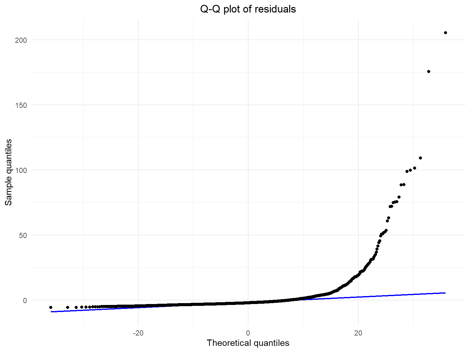

• The Q-Q plot of the residuals shows that the residual quantiles do not coincide with the theoretical quantiles in the right tail.

# Residual vs fitted value plot
ggplot(data.frame(Fitted = fitted(lrmodel), Residuals = residuals), aes(x = Fitted, y = Residuals)) +
  geom_point() +
  geom_hline(yintercept = 0, color = "blue") +
  labs(x = "Fitted values", y = "Residuals", title = "Residual vs. fitted values")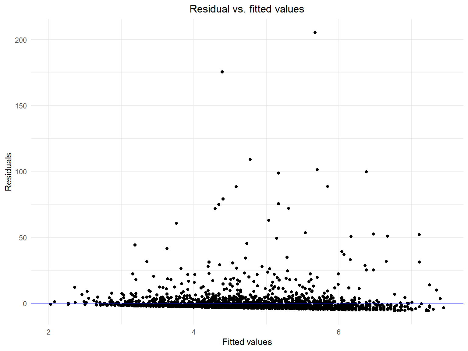

The plot of residuals versus fitted values reflects several problems:

• Ideally, the residuals should be randomly dispersed around the horizontal line (y = 0). In this plot, while there seems to be some level of randomness, there is a noticeable pattern where the residuals are not evenly distributed across the range of fitted values. This suggests that the model may not be capturing all the relevant patterns in the data.
• Residuals clustering: The clustering of residuals around certain ranges of fitted values indicates potential issues with the model. It might be missing some key predictive information or nonlinear relationships.
• Outliers: There seem to be several points that stand out from the general scatter of the residuals. These outliers can have a significant impact on the regression model, potentially skewing the results.
• Homoscedasticity check: The homoscedasticity assumption of linear regression means the residuals should have constant variance across all levels of fitted values. The spread of residuals in this plot does not appear to be uniform, suggesting the presence of heteroscedasticity, which violates this assumption.

The analysis of the residual Q-Q plot, and residuals vs. fitted values suggest that the linear regression model previously built may not be a good fit for the data.

Conclusion

• In this regression session of our entire work, we attempt to use the multiple linear regression to fit the data. The response variable is net_worth, and the predictors include age, gender, gdp_country, life_expectancy_countryand self_made. According to the model results, while age and the GDP of a billionaire’s country appear to have a significant association with their net worth, the overall model explains very little of the variation in net worth,i.e.,with a low adjusted R-squared value 0.0057, indicating that there are likely many other factors at play. At the same time, the analysis of residuals shows that the residuals do not have a zero mean and equal variance with several outliers, which violates the assumption of linear regression.
• In summary, the multiple linear regression model, as configured in our analysis, is not a good way to fit the data and predict the net worth of billionaires. This inadequacy could be attributed to the simplicity of our linear model, suggesting that there are numerous avenues for refinement and enhancement. Additionally, it may be the case that the net worth does not have a linear relationship with the predictors used in our model. Exploring alternative modeling methods that better capture the underlying relationships in the data is a topic for future research.

Discussion

In the exploratory analyses, we found that the majority of billionaires possess assets concentrated within the range of $1-5 billion, with few with assets over $100 billion. This is a bit unexpected, as we anticipated a more evenly distributed wealth among billionaires. Looking into the demographic characteristics of billionaires, we found a gap in the number of billionaires in different gender groups: female billionaires are much fewer than male billionaires. This result is similar to what we expected, given the glass ceiling effect that women have encountered; there are many factors preventing women from advancing to higher positions. The billionaires’ wealth patterns differ in factors such as age and industry: the average net wealth tends to increase as the age of the group increases, and Finance, Technology, and Manufacturing are the top three industries with the most billionaires in 2023.

Our examination of billionaires’ geographic distribution revealed the United States as the primary residence for the most billionaires, followed by China and the United Kingdom. Zooming in on the USA and China, a comparison of the top 10 billionaires in the two countries indicates a significant wealth disparity, with the top 10 billionaires in the USA possessing greater wealth than their Chinese counterparts. Additionally, GDP trends depict an overall upward trajectory, disrupted by a 2020 downturn in the USA likely linked to the COVID-19 pandemic.

Further analysis using longitudinal data allowed us to discern the impact of COVID-19 in more detail. The noticeable downturn in 2020 affected billionaires across all sectors, reflecting the pandemic’s adverse effects. Specifically focusing on the US, the GDP trend across almost all industries declined in 2020, indicating the widespread negative impact of COVID-19 on the nation’s economy. While our report initially didn’t center on analyzing the effects of COVID-19, the observation of its influence on diverse industries and the wealthiest individuals globally, underscores the evident impact of the epidemic and its aftermath on the world at large.

Following our exploratory analyses, we performed hypothesis tests to determine the statistical significance of observed patterns or trends. As anticipated, we found a significant increase in billionaires’ wealth from 2010 to 2023, with a 95% confidence interval indicating a true increase ranging between $2.6 and 4.3 billion. Additionally, we verified the wealth difference in age groups using the transformed data. Notably, while there exists a substantial gap between the number of male and female billionaires, our test results indicate that the average net worth of each group does not exhibit statistical disparity.

Finally, we wanted to see if any factors contribute to the wealth accumulation of billionaires. Hence, we focused on billionaires in 2023 and fit a linear regression model. We identified age and country GDP as potential factors influencing wealth accumulation. The regression model revealed coefficients of 0.0485 for age and 0.0565 for country GDP. It suggests that holding other factors constant, each additional year of age contributes to the increase in a billionaire’s net worth by roughly 0.0485 billion, and every unit rise in the country’s GDP contributes to that by 0.0565 billion. However, as already discussed in the Regression section of this report, our model has some limitations. The adjusted R-squared implies that only 0.6% of the variance in the net worth of billionaires is captured by the model, indicating we are missing some key predictive information. Moreover, the original data fails to meet the assumptions of homoscedasticity and normal distribution of residuals, which makes the result less robust. Some further improvements would be to include additional predictors or explore alternative modeling methods that better capture the underlying relationships in the data.

---

Copyright © P8105, Fall 2023